Machine Learning and Neural Networks
Roberto Santana and Unai Garciarena
Department of Computer Science and Artificial Intelligence
University of the Basque Country
Mathematical background for deep learning: Table of Contents
Data generating process
Definitions
- Data generating process: We assume this is the (true) process from which training and test datasets are generated.
- Data generating distribution: This is the probability distribution of the data determined by generating process: \(p_{data}\).
Example
- The relationship between \(n\) protein expressions, \( x_1, \dots, x_n \) and a diagnostic \(y \in \{0,1\}\) variable.
- The genetic process has its own rules that determine the relationship between the protein expressions and the diagnostic.
- This genetic process also defines data distributions \(p(x,y)\) and \(p(y|x)\).
Data generating process and model families
- Model: Specifies which functions ( model family) the learning algorithm can choose from when varying the parameters in order to approximate the data generating process.
- Model capacity: Its capacity to fit a wide variety of functions.
- Hypothesis space: The set of functions that the learning algorithm is allowed to select as being the solution.
Data generating process and model families
Example: Linear models of different capacity
- Linear regression model: \[ \hat{y} = b + w {\bf{x}} \]
- Linear regression model quadratic as a function of \( {\bf{x}} \): \[ \hat{y} = b + w_1 {\bf{x}} + w_2 {\bf{x}}^2 \]
- Linear regression model, polynomial of degree \(9\): \[ \hat{y} = b + \sum_{i=1}^{9} w_i {\bf{x}}^i \]
I. Goodfellow and Y. Bengio and A. Courville. Deep Learning.. MIT Press. 2016.
Data generating process and model families
- Situations for a model family being trained:
- Excluded the true data generating process.
- Matched the true data generating process.
- Included the generating process but also many other possible generating processes.
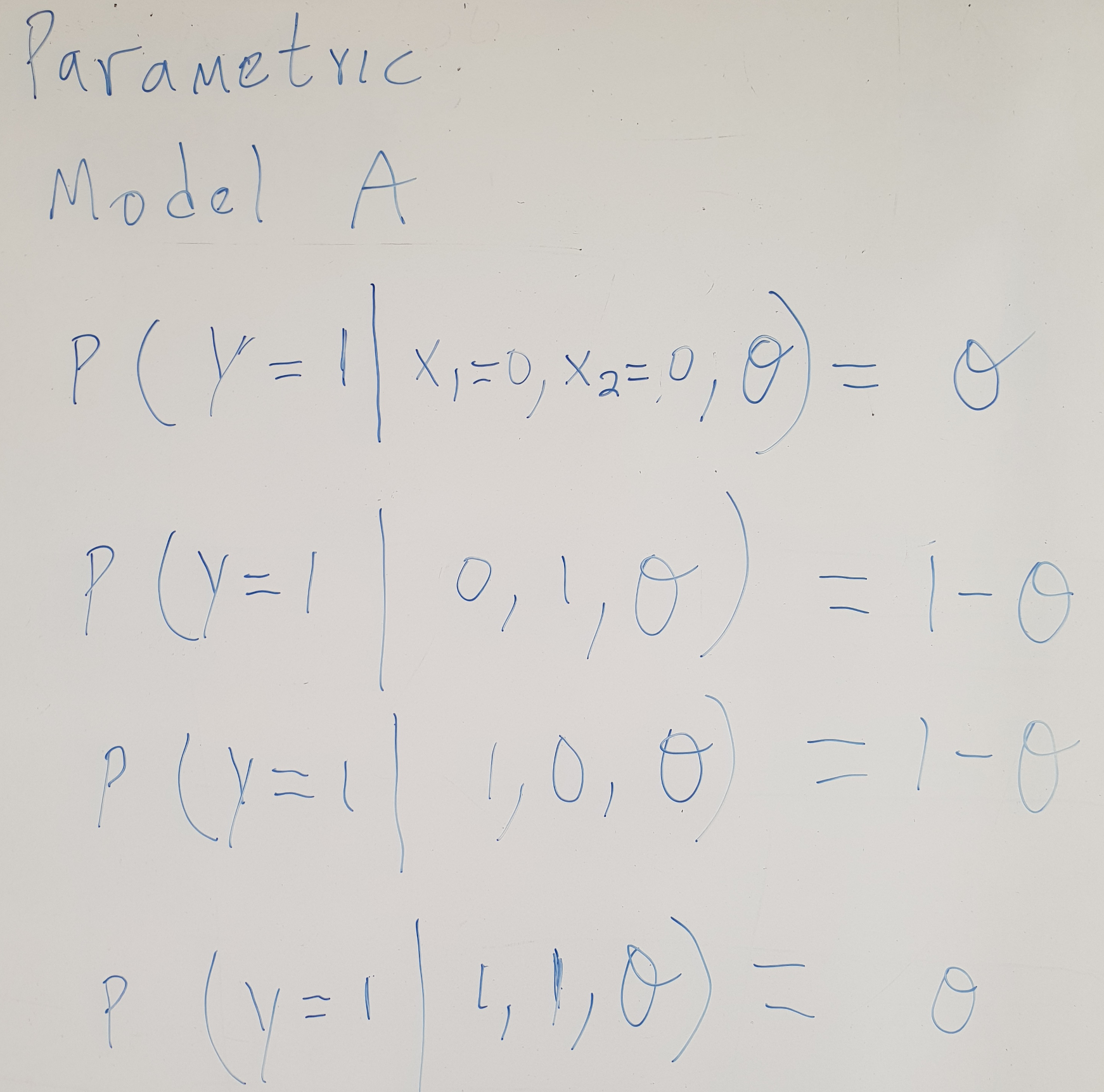
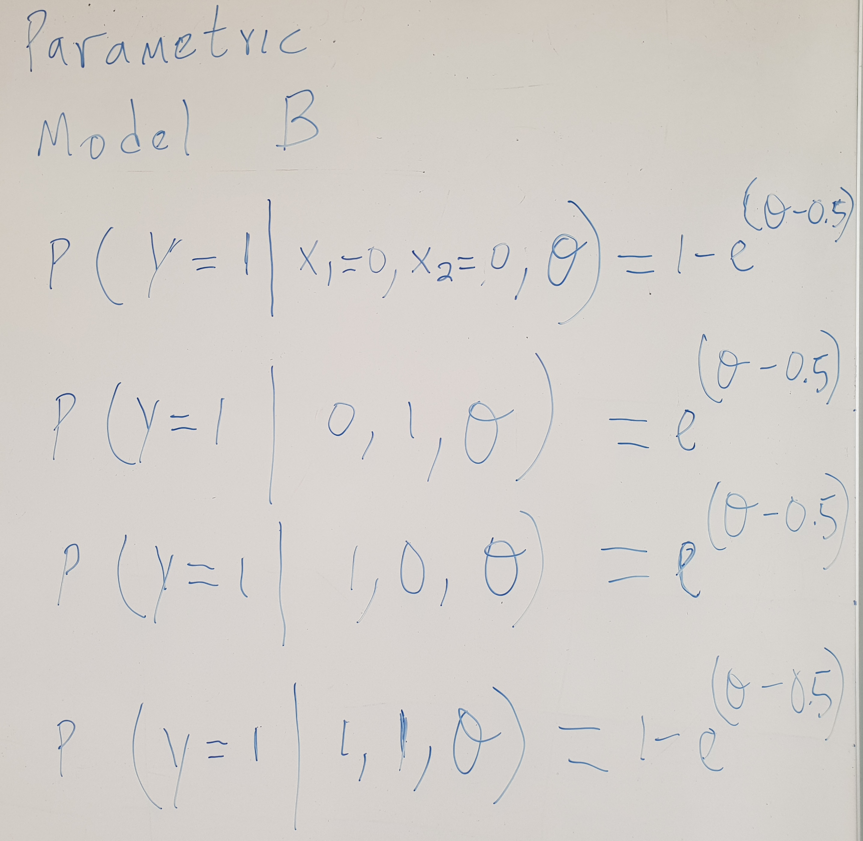
Find the model best suited for the data
Find the model best suited for the data
Find the model best suited for the data
How likely are the models for the data?
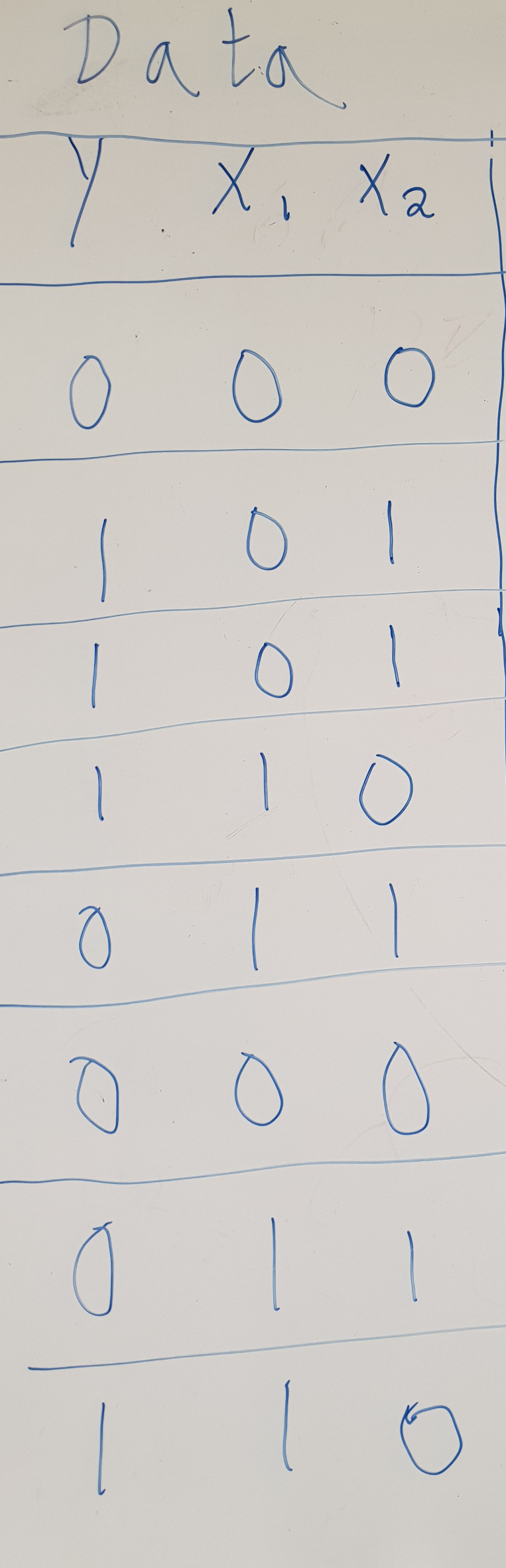
| Data | Model 1 | Model 2 | Model 3 |
|---|---|---|---|
| \(y x_1 x_2\) | \(p_{M1}(y|x_1,x_2) \) | \(p_{M2}(y|x_1,x_2) \) | \(p_{M3}(y|x_1,x_2) \) |
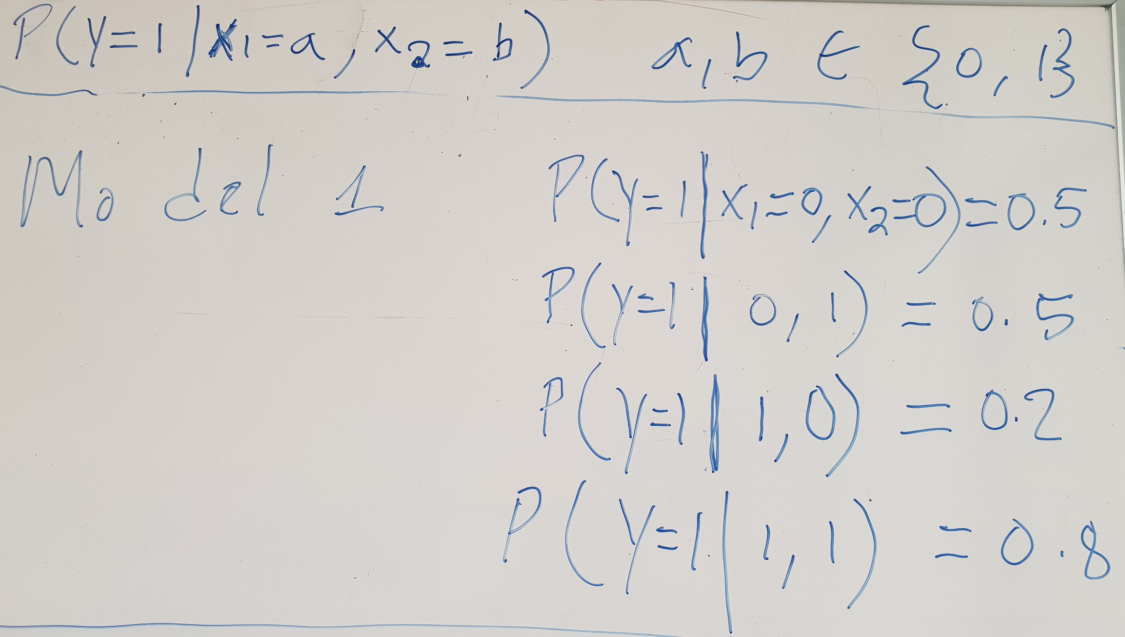
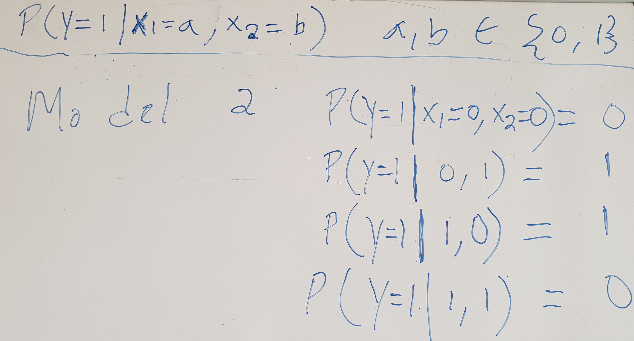
| 000 | 0.5 | 1.0 | 1.0 |
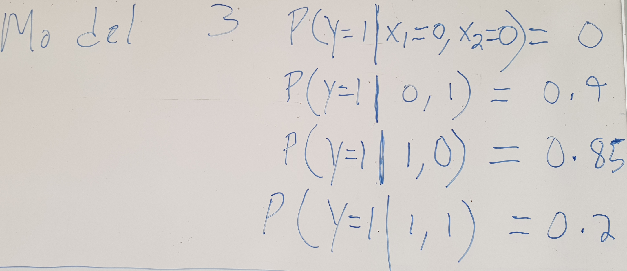
| 101 | 0.5 | 1.0 | 0.9 |
| 101 | 0.5 | 1.0 | 0.9 |
| 110 | 0.2 | 1.0 | 0.85 |
| 011 | 0.2 | 1.0 | 0.8 |
| 000 | 0.5 | 1.0 | 1.0 |
| 011 | 0.2 | 1.0 | 0.8 |
| 110 | 0.2 | 1.0 | 0.85 |
How likely are the models for the data?
| Data | Model 1 | Model 2 | Model 3 |
|---|---|---|---|
| \(y x_1 x_2\) | \(p_{M1}(y|x_1,x_2) \) | \(p_{M2}(y|x_1,x_2) \) | \(p_{M3}(y|x_1,x_2) \) |
| 000 | 0.5 | 1.0 | 1.0 |
| 101 | 0.5 | 1.0 | 0.9 |
| 101 | 0.5 | 1.0 | 0.9 |
| 110 | 0.2 | 1.0 | 0.85 |
| 011 | 0.2 | 1.0 | 0.8 |
| 000 | 0.5 | 1.0 | 1.0 |
| 011 | 0.2 | 1.0 | 0.8 |
| 110 | 0.2 | 1.0 | 0.85 |
| \(\prod_{i=1}^{8} p(y|x_1,x_2) \) | \(0.2^4*0.5^4\) | 1.0 | \(0.85^2*0.8^2*0.9^2\) |
| \(log(\prod_{i=1}^{8} p(y|x_1,x_2)) \) | \(log(0.2^4*0.5^4)\) | \(log(1.0)\) | \(\log(0.85^2*0.8^2*0.9^2 )\) |
| \(\sum_{i=1}^{8} log(p(y|x_1,x_2)) \) | \(4*log(0.2)+4*log(0.5)\) | \(0 \) | \(2*\log(0.85)+2*log(0.8)+2*log(0.9)\) |
Find the model best suited for the data
Estimators, Bias and Variance
Estimators
- Point estimation is the attempt to provide "the best" prediction for a quantity of interest, e.g., the parameters of a ML model.
- A point estimator is a any function of the data \( \hat{\theta}_m = g({\bf{x}}^1, \dots,{\bf{x}}^m) \).
- A good estimator is a function whose output is close to the true underlying \(\theta\) that generated the training data.
- We assume that the true parameter of \(\theta\) is true but unknown. Therefore, \( \hat{\theta} \) is a random variable.
- Function estimator (\( \hat{f}\)): When the goal is to estimate the relationship between input and target variables.
Estimators
Estimators, Bias and Variance
Bias
- The bias of an estimator is defined as: \[ bias(\hat{\theta}_m) = \mathbb{E}(\hat{\theta}_m) -\theta, \]
- An estimator is said to be unbiased if \( bias(\hat{\theta}_m)=0 \) .
- An estimator is said to be asymptotically unbiased if \[ lim_{m \leftarrow infty} bias(\hat{\theta}_m)=0 \]
where the expectation is over the data (samples of the random variable).
Estimators
Estimators, Bias and Variance
Bias
- We compute the bias for the Bernoulli distribution with parameter \( \theta \) :
\[ P({\bf{x}};\theta) = \theta^{\bf{x}} (1-\theta)^{(1-{\bf{x}})}. \] - Having a set of samples \( \{ x^1, \dots, x^m \} \), a common estimator for \( \theta \) is the mean of the training samples: \[ \hat{\theta_m} = \frac{1}{m} \sum_{i=1}^{m} x^i. \]
- For this estimator, we will compute \( bias(\hat{\theta}_m) = \mathbb{E}(\hat{\theta}_m) -\theta \).
Estimators, Bias and Variance
Bias
\[ \begin{align} bias(\hat{\theta}_m) &=& \mathbb{E}(\hat{\theta}_m) -\theta \\ &=& \mathbb{E} \left [ \frac{1}{m} \sum_{i=1}^{m} x^i \right ] - \theta \\ &=& \frac{1}{m} \sum_{i=1}^{m} \mathbb{E} [x^i] - \theta \\ &=& \frac{1}{m} \sum_{i=1}^{m} \sum_{x^i=0}^{1} \left (x^i \theta^{x^i} (1-\theta)^{(1-x^i)} \right) - \theta \\ &=& \frac{1}{m} \sum_{i=1}^{m}(\theta) - \theta \\ &=& 0 \end{align} \]
Estimators, Bias and Variance
Variance
- The variance of an estimator is defined as: \[ Var(\hat{\theta}_m) \]
It provides information about how much we expect the estimator to vary as a function of the data sample.
Estimators, Bias and Variance
Variance
- The square root of the variance is called the standard error.
- The standard error of the mean is given by: \[ SE(\hat{\mu}_m) = \sqrt{Var \left [ \frac{1}{m} \sum_{i=1}^{m} x^i \right]} = \frac{\sigma}{\sqrt{m}} \] where \(\sigma^2 \) is the true variance of the samples.
Estimators
Estimators, Bias and Variance
Example: Variance of the sample mean for Benoulli distribution
- The variance of this estimator decreases as a function of \(m\).
\[ \begin{align} Var(\hat{\theta}_m) &=& Var \left ( \frac{1}{m} \sum_{i=1}^{m} x^i \right ) \\ &=& \frac{1}{m^2} \sum_{i=1}^{m} Var (x^i) \\ &=& \frac{1}{m^2} \sum_{i=1}^{m} \theta (1-\theta) \\ &=& \frac{1}{m^2} m \theta (1-\theta) \\ &=& \frac{1}{m} \theta (1-\theta) \\ \end{align} \]
Maximum Likelihood Estimation (MLE)
- We consider a set of \(m\) samples \( \mathbb{X} = \{ {{\bf{x}}}^1, \dots, {\bf{x}}^m \} \) drawn independently from the true but unknown data generating distribution \(p_{data}({{\bf{x}}})\).
- \( p_{model}({\bf{x}},\theta) \) is a parametric family of probability distributions over the same space indexed by \(\theta\).
- The maximum likelihood estimator for \(\theta\) is defined as: \[ \begin{align} \theta_{ML} &=& \underset{\theta}{\arg\max} \prod_{i=1}^{m} p_{model}(\mathbb{X},\theta)\\ &=& \underset{\theta}{\arg\max} \prod_{i=1}^{m} p_{model}({\bf{x}}^i,\theta) \end{align} \]
Maximum Likelihood Estimation (MLE)
- Usually, the logarithm is used to transform the product of probabilities to a sum of logarithms: \[ \theta_{ML} = \underset{\theta}{\arg\max} \sum_{i=1}^{m} log \; p_{model}({\bf{x}}^i,\theta) \]
- This is an equivalent optimization problem that can be also expressed as an optimization as an expectation with respect to the empirical distribution \(\hat{p}_{data}\): \[ \theta_{ML} = \underset{\theta}{\arg\max} \; \mathbb{E}_{{\bf{x}} \thicksim \hat{p}_{data}} log \; p_{model}({\bf{x}},\theta) \]
I. Goodfellow and Y. Bengio and A. Courville. Deep Learning.. MIT Press. 2016.
Maximum Likelihood Estimation (MLE)
Kullback Leibler divergence interpretation
- The MLE can be also seen from the perspective of the Kullback-Leibler divergence between two distributions: \[ D_{KL}(\hat{p}_{data}||p_{model}) = \mathbb{E}_{{\bf{x}} \thicksim \hat{p}_{data}} \left [ log \; \hat{p}_{data}({\bf{x}})-log \; p_{model}({\bf{x}}) \right ] \]
- Since \(\hat{p}_{data}({\bf{x}})\) does not depend on the model selection, we only need to minimize: \[ - \underset{\theta}{\arg\max} \; \mathbb{E}_{{\bf{x}} \thicksim \hat{p}_{data}} \left [log \; p_{model}({\bf{x}}) \right ] \]
- Therefore, minimizing the KL divergence corresponds to minimizing the cross-entropy between the distributions.
I. Goodfellow and Y. Bengio and A. Courville. Deep Learning.. MIT Press. 2016.
Maximum Likelihood Estimation (MLE)
Conditional probability
- The MLE can be also applied to the estimation of the conditional probability \( P(y| {\bf{x}},\theta) \): \[ \theta_{ML} = \underset{\theta}{\arg\max} \prod P(\mathbb{Y}| \mathbb{X},\theta) \]
- If the instances are assumed to be i.i.d., then the expression can be decomposed into: \[ \theta_{ML} = \underset{\theta}{\arg\max} \sum_{i=1}^{m} log \; P(y^i|{\bf{x}}^i,\theta). \]
I. Goodfellow and Y. Bengio and A. Courville. Deep Learning.. MIT Press. 2016.
How likely are the models for the data?
| Data | Model 1 | Model 2 | Model 3 |
|---|---|---|---|
| \(y x_1 x_2\) | \(p_{M1}(y|x_1,x_2) \) | \(p_{M2}(y|x_1,x_2) \) | \(p_{M3}(y|x_1,x_2) \) |
| 000 | 0.5 | 1.0 | 1.0 |
| 101 | 0.5 | 1.0 | 0.9 |
| 101 | 0.5 | 1.0 | 0.9 |
| 110 | 0.2 | 1.0 | 0.85 |
| 011 | 0.2 | 1.0 | 0.8 |
| 000 | 0.5 | 1.0 | 1.0 |
| 011 | 0.2 | 1.0 | 0.8 |
| 110 | 0.2 | 1.0 | 0.85 |
| \(\prod_{i=1}^{8} p(y|x_1,x_2) \) | \(0.2^4*0.5^4\) | 1.0 | \(0.85^2*0.8^2*0.9^2\) |
| \(log(\prod_{i=1}^{8} p(y|x_1,x_2)) \) | \(log(0.2^4*0.5^4)\) | \(log(1.0)\) | \(\log(0.85^2*0.8^2*0.9^2 )\) |
| \(\sum_{i=1}^{8} log(p(y|x_1,x_2)) \) | \(4*log(0.2)+4*log(0.5)\) | \(0 \) | \(2*\log(0.85)+2*log(0.8)+2*log(0.9)\) |
Find the model best suited for the data
Maximum Likelihood Estimation (MLE)
Linear regression as an example
- We assume that in an infinitively large training set, there might be several training examples with the same input value \( {\bf{x}} \) but different values of \(y\).
- The goal of the learning algorithm is to fit the distribution \( p(y|{\bf{x}}) \) to all of those different \(y\) values compatible with \( {\bf{x}} \).
- We assume that \( p(y|{\bf{x}}) \) follows a Normal distribution \( p(y|{\bf{x}})= \mathcal{N}(y;\hat{y}({\bf{x}},w), \sigma^2)\).
- The function \(\hat{y}({\bf{x}},w) \) gives the prediction of the mean of the Gaussian.
- The variance is fixed to some constant \(\sigma^2\).
I. Goodfellow and Y. Bengio and A. Courville. Deep Learning.. MIT Press. 2016.
Maximum Likelihood Estimation (MLE)
Linear regression as an example
- For the Gaussian distribution: \[ \begin{align} P(y| {\bf{x}},\theta) &=& \mathcal{N}(y;\hat{y}({\bf{x}},w), \sigma^2) \\ &=& \frac{1}{\sqrt{2\pi \sigma^2}} -e^\frac{(y-\hat{y}({\bf{x}},w))^2}{2 \sigma^2} \end{align} \]
- Therefore, the conditional log-likelihood is given by: \[ \begin{align} \sum_{i=1}^{m} log \; P(y^i|{\bf{x}}^i,\theta) &=& \sum_{i=1}^{m} log \; \frac{1}{\sqrt{2\pi \sigma^2}} -e^\frac{(y^i-\hat{y}({\bf{x}}^i,w))^2}{2 \sigma^2} \\ &=& -m \, log(\sigma) - \frac{m}{2} log(2\pi) - \sum_{i=1}^{m} \frac{||\hat{y}^i-y^i||^2}{2\sigma^2} \end{align} \]
I. Goodfellow and Y. Bengio and A. Courville. Deep Learning.. MIT Press. 2016.
Maximum Likelihood Estimation (MLE)
Linear regression as an example
Maximizing the conditional likelihood \[ \sum_{i=1}^{m} log \; P(y^i|{\bf{x}}^i,\theta) = -m \, log(\sigma) - \frac{m}{2} log(2\pi) - \sum_{i=1}^{m} \frac{||\hat{y}^i-y^i||^2}{2\sigma^2} \]
is equivalent to minimizing the mean squared error: \[ MSE_{train} = \frac{1}{m} \sum_{i=1}^{m} ||\hat{y}^i-y^i||^2 \]
I. Goodfellow and Y. Bengio and A. Courville. Deep Learning.. MIT Press. 2016.
Maximum Likelihood Estimation (MLE)
Properties
- Under appropriate conditions, the maximum likelihood estimator has the property of consistency, i.e., as the number of training examples approaches infinity, the ML estimator of a parameter converges to the true value of the parameter.
- These conditions are:
- The true distribution \(p_{data}\) must lie within the model family \(p_{model}(.,\theta) \). Otherwise, no estimator can recover \(p_{data}\).
- The true distribution \(p_{data}\) must correspond to exactly one value of \( \theta \). Otherwise, maximum likelihood can recover the correct \(p_{data}\), but will not be able to determine which value of \( \theta \) was used by the data generating processing.
I. Goodfellow and Y. Bengio and A. Courville. Deep Learning.. MIT Press. 2016.
Differences between frequentist and Bayesian approaches
Bayesian approach
- The dataset is directly observed and therefore is not random.
- The true parameter \(\theta\) is unknown or uncertain and thus is represented as a random variable.
- The knowledge about \(\theta\), before observing the data, is represented using a prior probability distribution \( p(\theta)\).
Frequentist approach
- MLE follows a frequentist approach.
- The true parameter \(\theta\) is fixed but unknown.
- The point estimate \( \hat{\theta} \) is a random variable.
- It can be more convenient than Bayesian approaches when the number of training samples is large.
I. Goodfellow and Y. Bengio and A. Courville. Deep Learning.. MIT Press. 2016.
Bayesian approach
Bayes rule
- The way to update our belief about \(\theta\) using a set of data samples \( \{ {\bf{x}}^1, \dots, {\bf{x}}^m \} \) is by combining the the data likelihood \( p({\bf{x}}^1, \dots, {\bf{x}}^m |\theta)\) with the prior via the Bayes rule:
\[ p(\theta| {\bf{x}}^1, \dots, {\bf{x}}^m) = \frac{ p({\bf{x}}^1, \dots, {\bf{x}}^m|\theta)p(\theta)} {p({\bf{x}}^1, \dots, {\bf{x}}^m)} \] - The prior has an influence by shifting the probability mass density towards region of the parameter space that are preferred a priori.
I. Goodfellow and Y. Bengio and A. Courville. Deep Learning.. MIT Press. 2016.
Maximum A Posteriori (MAP) Estimation
- Even using the Bayesian approach, in some scenarios is convenient to compute a point estimate.
- The MAP estimate chooses the point of maximal posterior probability (or probability density for continuous \( \theta \)):
\[ \theta_{MAP} = \underset{\theta}{\arg\max} \;p(\theta|{\bf{x}}) = \underset{\theta}{\arg\max} \; log \, p({\bf{x}}|\theta) + log \, p(\theta) \] - The MAP estimate has the advantage of leveraging information that is brought by the prior and cannot be found in the training data.
I. Goodfellow and Y. Bengio and A. Courville. Deep Learning.. MIT Press. 2016.
Regularization
Important concepts
- Generalization: The ability of a model to perform well on previously unobserved inputs.
- The generalization error is defined as the expected value of the error on a new input.
- The expected error is usually estimated using a test set of examples.
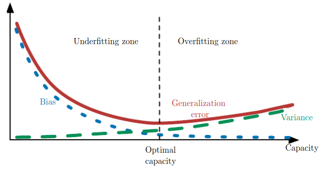
- Underfitting: Occurs when the model is not able to obtain a sufficiently low error value on the training set.
- Overfitting: Occurs when the gap between the training error and test error is too large.
I. Goodfellow and Y. Bengio and A. Courville. Deep Learning.. MIT Press. 2016.
Data generating process and model families
- Situations for a model family being trained:
- Excluded the true data generating process.
- Matched the true data generating process.
- Included the generating process but also many other possible generating processes.
Capacity, underfitting, overfitting
Regularization
- Regularization is any modification we make to a learning algorithm that is intended to reduce its generalization error but not its training error.
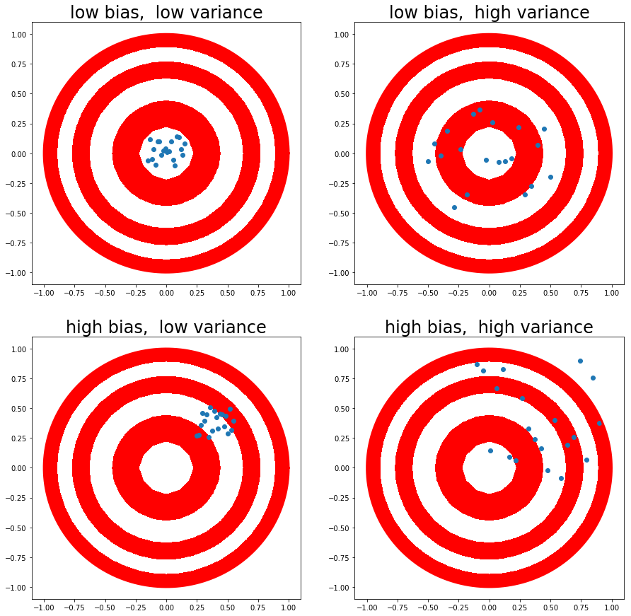
- Regularization of an estimator works by trading increased bias for reduced variance.
- An effective regularizer is one that reduces variance significantly by not overly increasing the bias.
- The goal is to achieve a model of sufficient complexity to fit the training data but able to generalize to unseen data.
I. Goodfellow and Y. Bengio and A. Courville. Deep Learning.. MIT Press. 2016.
Regularization
Parameter norm penalties
- Parameter regularization is implemented by adding a parameter norm penalty \(\Omega(\theta)\) to the objective function \(J\).
- The regularized objective function \(\tilde{J}\) is defined as:
\[ \tilde{J}(\theta;{\bf{X}},y) = J(\theta;{\bf{X}},y) + \alpha \, \Omega(\theta), \]
where \(\alpha \in [0,\infty] \) is a hyperparameter that weights the relative contribution of \(\Omega(\theta)\) relative to \( J(\theta;{\bf{X}},y) \).
I. Goodfellow and Y. Bengio and A. Courville. Deep Learning.. MIT Press. 2016.
Regularization
\(L^2\) parameter regularization
- The \(L^2\) parameter regularization adds a regularization term of the form \(\Omega(\theta) =\frac{1}{2} \Vert \theta \Vert_2^2 \).
- \(L^2\) adds squared magnitude of coefficient as penalty term.
- In neural networks, usually regularization is applied to the weights of network, i.e., \( \theta = w \).
- A regularized model of this type has the form:
\[ \tilde{J}(\theta;{\bf{X}},y) = J(\theta;{\bf{X}},y) + \frac{\alpha}{2} w^{\top}w. \]
I. Goodfellow and Y. Bengio and A. Courville. Deep Learning.. MIT Press. 2016.
Regularization
\(L^1\) parameter regularization
- The \(L^1\) parameter regularization adds a regularization term of the form:
\[ \Omega(\theta) = \Vert \theta \Vert_1 = \sum_i |w_i|. \] - A regularized model of this type has the form:
\[ \tilde{J}(\theta;{\bf{X}},y) = J(\theta;{\bf{X}},y) + \alpha \Vert \theta \Vert_1 \] - \(L^1\) adds absolute value of magnitude of coefficient as penalty term.
- \(L^1\) parameter regularization tends to produce more sparse solutions, i.e., some parameters have an optimal value of zero.
I. Goodfellow and Y. Bengio and A. Courville. Deep Learning.. MIT Press. 2016.